

Classification of the urinary metabolome using machine learning and potential applications to diagnosing interstitial cystitis

With the advent of artificial intelligence (AI) in biostatistical analysis and modeling, machine learning can potentially be applied into developing diagnostic models for interstitial cystitis (IC). In the current clinical setting, urologists are depen-dent on cystoscopy and questionnaire-based decisions to diagnose IC. This is a result of a lack of objective diagnostic molecular biomarkers. The purpose of this study was to develop a machine learning-based method for diagnosing IC and assess its performance using metabolomics profiles obtained from a prior study. To develop the machine learning algorithm, two classification methods, support vector machine (SVM) and logistic regression (LR), set at various pa-rameters, were applied to 43 IC patients and 16 healthy controls. There were 3 measures used in this study, accuracy, precision (positive predictive value), and recall (sensitivity). Individual precision and recall (PR) curves were drafted. Since the sample size was relatively small, complicated deep learning could not be done. We achieved a 76%–86% accuracy with leave-one-out cross validation depending on the method and parameters set. The highest accuracy achieved was 86.4% using SVM with a polynomial kernel degree set to 5, but a larger area under the curve (AUC) from the PR curve was achieved using LR with a l1-norm regularizer. The AUC was greater than 0.9 in its ability to discriminate IC patients from controls, suggesting that the algorithm works well in identifying IC, even when there is a class distribution imbal-ance between the IC and control samples. This finding provides further insight into utilizing previously identified urinary metabolic biomarkers in developing machine learning algorithms that can be applied in the clinical setting.
INTRODUCTION
MATERIALS AND METHODS
Ethics statement
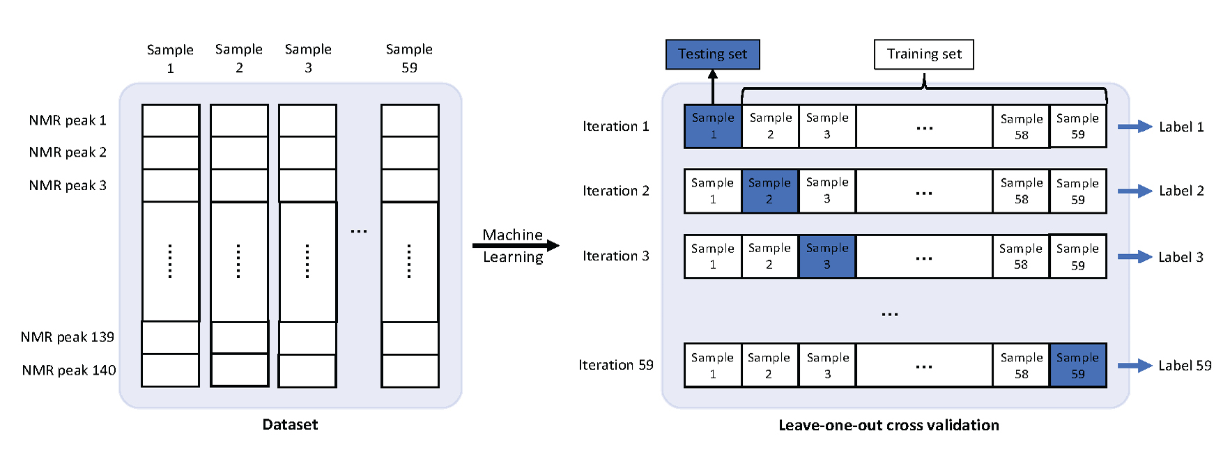
Dataset
Method
Training
Evaluation
RESULTS
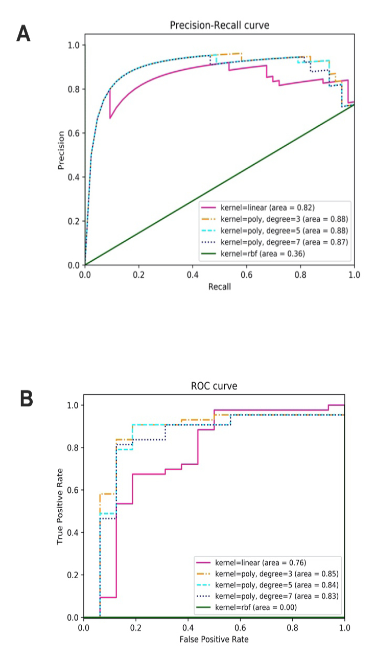
Classification of IC samples with SVM
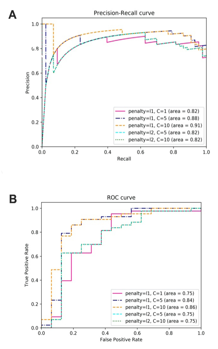
Classification of IC samples with LR
| Parameters | TP | TN | FP | FN | Accuracy | Precision | Recall | AUC of PR | AUC of ROC |
|---|---|---|---|---|---|---|---|---|---|
| Kernel = linear | 36 | 9 | 7 | 7 | 0.763 | 0.837 | 0.837 | 0.82 | 0.76 |
| Kernel = poly, degree = 3 | 39 | 11 | 5 | 4 | 0.847 | 0.886 | 0.907 | 0.88 | 0.85 |
| Kernel = poly, degree = 5 | 39 | 12 | 4 | 4 | 0.864 | 0.907 | 0.907 | 0.88 | 0.84 |
| Kernel = poly, degree = 7 | 39 | 11 | 5 | 4 | 0.847 | 0.886 | 0.907 | 0.87 | 0.83 |
| Kernel = RBF | 43 | 0 | 16 | 0 | 0.729 | 0.729 | 1.000 | 0.36 | 0.00 |
| LR | TP | TN | FP | FN | Accuracy | Precision | Recall | AUC of PR | AUC of ROC |
|---|---|---|---|---|---|---|---|---|---|
| Penalty = l1, C = 1 | 39 | 9 | 7 | 4 | 0.814 | 0.848 | 0.907 | 0.82 | 0.75 |
| Penalty = l1, C = 5 | 39 | 10 | 6 | 4 | 0.831 | 0.867 | 0.907 | 0.88 | 0.84 |
| Penalty = l1, C = 10 | 38 | 12 | 4 | 5 | 0.847 | 0.905 | 0.884 | 0.91 | 0.86 |
| Penalty = l2, C = 5 | 38 | 7 | 9 | 5 | 0.763 | 0.809 | 0.884 | 0.82 | 0.75 |
| Penalty = l2, C = 10 | 38 | 7 | 9 | 5 | 0.763 | 0.809 | 0.884 | 0.82 | 0.75 |
DISCUSSION
-
-
Hanno P, Keay S, Moldwin R, Van Ophoven A (2005) International Consultation on IC - Rome, September 2004/Forging an International Consensus: progress in painful bladder syndrome/interstitial cystitis. Report and abstracts. Int Urogynecol J Pelvic Floor Dysfunct 16 Suppl 1: S2-S34. [PubMed] [Google Scholar]
-
Nordling J, Anjum FH, Bade JJ, Bouchelouche K, Bouchelouche P, et al. (2004) Primary evaluation of patients suspected of having interstitial cystitis (IC). Eur Urol 45: 662-669.doi: https://doi.org/10.1016/j.eururo.2003.11.021. [View Article] [PubMed] [Google Scholar]
-
Hanno PM, Burks DA, Clemens JQ, Dmochowski RR, Erickson D, et al. (2011) AUA guideline for the diagnosis and treatment of interstitial cystitis/bladder pain syndrome. J Urol 185: 2162-2170.doi: https://doi.org/10.1016/j.juro.2011.03.064. [View Article] [PubMed] [Google Scholar]
-
Urinology Think Tank Writing Group (2018) Urine: Waste product or biologically active tissue. Neurourol Urodyn 37: 1162-1168.doi: https://doi.org/10.1002/nau.23414. [View Article] [PubMed] [Google Scholar]
-
Wen H, Lee T, You S, Park S, Song H, et al. (2014) Urinary metabolite profiling combined with computational analysis predicts interstitial cystitis-associated candidate biomarkers. J Proteome Res 14: 541-548.doi: https://doi.org/10.1021/pr5007729. [View Article] [PubMed] [Google Scholar]
-
Kind T, Cho E, Park TD, Deng N, Liu Z, et al. (2016) Interstitial cystitis-associated urinary metabolites identified by mass-spectrometry based metabolomics analysis. Sci Rep 6: 39227.doi: https://doi.org/10.1038/srep39227. [View Article] [PubMed] [Google Scholar]
-
Shahid M, Lee MY, Yeon A, Cho E, Sairam V, et al. (2018) Menthol, a unique urinary volatile compound, is associated with chronic inflammation in interstitial cystitis. Sci Rep 8: 10859.doi: https://doi.org/10.1038/s41598-018-29085-3. [View Article] [PubMed] [Google Scholar]
-
Cahan EM, Hernandez-Boussard T, Thadaney-Israni S, Rubin DL (2019) Putting the data before the algorithm in big data addressing personalized healthcare. NPJ Digit Med 2: 78.doi: https://doi.org/10.1038/s41746-019-0157-2. [View Article] [PubMed] [Google Scholar]
-
Tolles J, Meurer WJ (2016) Logistic regression: relating patient characteristics to outcomes. JAMA 316: 533-534. [PubMed] [Google Scholar]
-
Cortes C, Vapnik V (1995) Support-vector networks. Machine learning 20: 273-97.doi: https://doi.org/10.1007/BF00994018. [View Article][Google Scholar]
-
Platt JC (1998) [Internet]. Microsoft Research. Sequential minimal optimization: A fast algorithm for training support vector machines. Available from: https://www.microsoft.com/en-us/research/wp-content/uploads/2016/02/tr-98-14.pdf.
-
Lin Y, Lee Y, Wahba G (2002) Support vector machines for classification in nonstandard situations. Mach Learn 46: 191-202.[Google Scholar]
-
Tibshirani R (1996) Regression shrinkage and selection via the lasso. J Roy Stat Soc B 58: 267-88.doi: https://doi.org/10.1111/j.2517-6161.1996.tb02080.x. [View Article][Google Scholar]
-
Ng AY (2004) Feature selection, L1 vs. L2 regularization, and rotational invariance. In: Proceedings of the twenty-first international conference on Machine learning. New York, NY: Association for Computing Machinery.doi: https://doi.org/10.1145/1015330.1015435. [View Article]
-
Vehtari A, Gelman A, Gabry J (2017) Practical Bayesian model evaluation using leave-one-out cross-validation and WAIC. Statistics and Computing 27: 1413-1432.doi: https://doi.org/10.1007/s11222-016-9696-4. [View Article][Google Scholar]
-
Esteva A, Robicquet A, Ramsundar B, Kuleshov V, DePristo M, et al. (2019) A guide to deep learning in healthcare. Nat Med 25: 24-29.doi: https://doi.org/10.1038/s41591-018-0316-z. [View Article] [PubMed] [Google Scholar]
-
Miotto R, Wang F, Wang S, Jiang X, Dudley JT (2018) Deep learning for healthcare: review, opportunities and challenges. Brief Bioinform 19: 1236-1246.doi: https://doi.org/10.1093/bib/bbx044. [View Article] [PubMed] [Google Scholar]
-
Zampieri G, Vijayakumar S, Yaneske E, Angione C (2019) Machine and deep learning meet genome-scale metabolic modeling. PLoS Comput Biol 15:doi: https://doi.org/10.1371/journal.pcbi.1007084. [View Article] [PubMed] [Google Scholar]
-
Bordbar A, Monk JM, King ZA, Palsson BO (2014) Constraint-based models predict metabolic and associated cellular functions. Nat Rev Genet 15: 107-120.doi: https://doi.org/10.1038/nrg3643. [View Article] [PubMed] [Google Scholar]
-
Cuperlovic-Culf M (2018) Machine Learning Methods for Analysis of Metabolic Data and Metabolic Pathway Modeling. Metabolites 8:doi: https://doi.org/10.3390/metabo8010004. [View Article] [PubMed] [Google Scholar]
-
Angermueller C, Pärnamaa T, Parts L, Stegle O (2016) Deep learning for computational biology. Mol Syst Biol 12: 878.doi: https://doi.org/10.15252/msb.20156651. [View Article] [PubMed] [Google Scholar]
-
Min S, Lee B, Yoon S (2017) Deep learning in bioinformatics. Brief Bioinform 18: 851-869.doi: https://doi.org/10.1093/bib/bbw068. [View Article] [PubMed] [Google Scholar]
-
Vamathevan J, Clark D, Czodrowski P, Dunham I, Ferran E, et al. (2019) Applications of machine learning in drug discovery and development. Nat Rev Drug Discov 18: 463-477.doi: https://doi.org/10.1038/s41573-019-0024-5. [View Article] [PubMed] [Google Scholar]
-
Jing Y, Bian Y, Hu Z, Wang L, Xie XS (2018) Deep learning for drug design: an artificial intelligence paradigm for drug discovery in the big data era. AAPS J 20: 58.doi: https://doi.org/10.1208/s12248-018-0210-0. [View Article] [PubMed] [Google Scholar]
-
Klauschen F, Muller KR, Binder A, Bockmayr M, Hagele M, et al. (2018) Scoring of tumor-infiltrating lymphocytes: From visual estimation to machine learning. Semin Cancer Biol 52: 151-157.doi: https://doi.org/10.1016/j.semcancer.2018.07.001. [View Article] [PubMed] [Google Scholar]
-
Baptista D, Ferreira PG, Rocha M (2020) Deep learning for drug response prediction in cancer. Brief Bioinform: pii: bbz171.doi: https://doi.org/10.1093/bib/bbz171. [View Article] [PubMed] [Google Scholar]
-
Tolios A, De Las Rivas J, Hovig E, Trouillas P, Scorilas A, et al. (2020) Computational approaches in cancer multidrug resistance research: Identification of potential biomarkers, drug targets and drug-target interactions. Drug Resistance Updates 48: 100662.doi: https://doi.org/10.1016/j.drup.2019.100662. [View Article] [PubMed] [Google Scholar]
-
Wong NC, Lam C, Patterson L, Shayegan B (2018) Use of machine learning to predict early biochemical recurrence after robot-assisted prostatectomy. BJU Int 123: 51-57.doi: https://doi.org/10.1111/bju.14477. [View Article] [PubMed] [Google Scholar]
-
Madhukar NS, Khade PK, Huang L, Gayvert K, Galletti G, et al. (2019) A Bayesian machine learning approach for drug target identification using diverse data types. Nat Commun 10: 5221.doi: https://doi.org/10.1038/s41467-019-12928-6. [View Article] [PubMed] [Google Scholar]
-
Saeed K, Rahkama V, Eldfors S, Bychkov D, Mpindi JP, et al. (2017) Comprehensive drug testing of patient-derived conditionally reprogrammed Cells from Castration-resistant prostate cancer. Eur Urol 71: 319-327.doi: https://doi.org/10.1016/j.eururo.2016.04.019. [View Article] [PubMed] [Google Scholar]
-